Kruskal–Wallis one-way analysis of variance
In statistics, the Kruskal–Wallis one-way analysis of variance by ranks (named after William Kruskal and W. Allen Wallis) is a non-parametric method for testing whether samples originate from the same distribution. It is used for comparing more than two samples that are independent, or not related. The parametric equivalence of the Kruskal-Wallis test is the one-way analysis of variance (ANOVA). The factual null hypothesis is that the populations from which the samples originate, have the same median. When the Kruskal-Wallis test leads to significant results, then at least one of the samples is different from the other samples. The test does not identify where the differences occur or how many differences actually occur. It is an extension of the Mann–Whitney U test to 3 or more groups.The Mann-Whitney would help analyze the specific sample pairs for significant differences.
Since it is a non-parametric method, the Kruskal–Wallis test does not assume a normal population, unlike the analogous one-way analysis of variance. However, the test does assume an identically-shaped and scaled distribution for each group, except for any difference in medians.
Contents |
Method
- Rank all data from all groups together; i.e., rank the data from 1 to N ignoring group membership. Assign any tied values the average of the ranks they would have received had they not been tied.
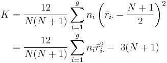
- The test statistic is given by:
 where:
 is the number of observations in group
 is the rank (among all observations) of observation
  from group
 is the total number of observations across all groups
 ,
, is the average of all the
  .
.
- Notice that the denominator of the expression for
 is exactly
  and
and  . Thus

Notice that the last formula only contains the squares of the average ranks.
- A correction for ties can be made by dividing
 by
by  , where G is the number of groupings of different tied ranks, and ti is the number of tied values within group i that are tied at a particular value. This correction usually makes little difference in the value of K unless there are a large number of ties.
 - Finally, the p-value is approximated by
 . If some
  values are small (i.e., less than 5) the probability distribution of K can be quite different from this chi-squared distribution. If a table of the chi-squared probability distribution is available, the critical value of chi-squared,
  , can be found by entering the table at g − 1 degrees of freedom and looking under the desired significance or alpha level. The null hypothesis of equal population medians would then be rejected if
  . Appropriate multiple comparisons would then be performed on the group medians.
 - If the statistic is not significant, then no differences exist between the samples. However, if the test is significant then a difference exists between at least two of the samples. Therefore, a researcher might use sample contrasts between individual sample pairs, or post hoc tests, to determine which of the sample pairs are significantly different. When performing multiple sample contrasts, the Type I error rate tends to become inflated.
See also
References
- Kruskal and Wallis. Use of ranks in one-criterion variance analysis. Journal of the American Statistical Association 47 (260): 583–621, December 1952. [1]
- Siegel and Castellan. (1988). "Nonparametric Statistics for the Behavioral Sciences" (second edition). New York: McGraw–Hill.
- Corder, Gregory W., and Dale I. Foreman. Nonparametric Statistics for Non-Statisticians. 1st ed. Hoboken: John Wiley & Sons, Inc., 2009. 99-105. Print.